GRASS for Viewsheds

Documenting some first steps with GRASS to do some geographical analysis for planning of radio installations. This was after some frustration at the clunkiness of on-line services like Hey What’s That. The only feasible alternative seemed to be to start using a proper GIS system ourselves and then try to make available the specific operations that we use so we don’t have to do all the analysis ourselves.

So the first step was to obtain some data to use as a background map so we can eyeball what we’re doing and some topological data. As academics we have access to both of these from the Ordnance Survey through EDINA. What we get from EDINA is the Master Map in either 1:10k or 1:25k resolution and the PROFILE DTM topological data at 1:10k resolution.

This data comes to us as a lot of small files. In the case of the background map it is tiny TIFF files together with some information about how each file maps onto the real-world coordinate system, in a separate file with a .tfw extension. To be able to display these in a GIS system, they have to be merged into one big tiff, which ought as well to use the extensions that allow it to carry some information about the coordinate system. We use the gdal_merge.py program for this.

gdal_merge.py -pct -o edinburgh_raster_10k.gtiff -of Gtiff raster-10k/*.tif

The -pct option means to grab the colour map from the first tiff file otherwise what you’ll eventually see is an unreadable dark greyscale image.

The next step is to import the data into GRASS’s internal format. The first thing to understand is that in this case though the GeoTIFF file now carries coordinate information, it doesn’t carry the information about which coordinate system or projection is being used. Because this data comes from the Ordnance Survey, we know it is British National Grid using the OSGB1936 datum a.k.a. EPSG:27700. This becomes important when combining with maps from other sources and making measurements such as distance.

In any event, we import the GeoTIFF file and create a new “location” called, in this case, Edinburgh. The “-o” flag causes GRASS to ignore the lack of projection information carried in the source file. The name of the command, r.in.gdal, means that it is about raster maps (r) and input (in) and uses the GDAL library that knows about working with these sorts of files.

r.in.gdal -o in=edinburgh_raster_10k.gtiff out=raster_10k location=Edinburgh

Now for the topological data. The default way to download it gives you an NTF file. This is a format that the Ordnance Survey uses and is a vector format, even though for the Digital Terrain Map it is basically point data. If you try using this GRASS will try to add all the millions of points to a spatial index. This will be very slow and probably use up all of the available RAM. It is better to download it as TIFF files. These can then be imported in the same way as described above.

gdal_merge -o edinburgh_profile_dtm.gtiff profile-dtm/*.tif
r.in.gdal -o in=edinburgh_profile_dtm.gtiff out=profile_dtm

It probably makes sense to do this first, before the background map. The reason being that the TIFF files one gets for the DTM data do contain projection information and coordinate system embedded, that is, they are GeoTIFF files. If the “location” is created from them, it will have the correct projection automatically.

Reading the Wiki page about Contour Lines to Digital Elevation Models, I wonder if it would not have been better to obtain the countour lines rather than the pre-computed DTM from EDINA. Perhaps not as we would have to compute the DTM ourselves in any case. Where might contour lines be more useful on their own?

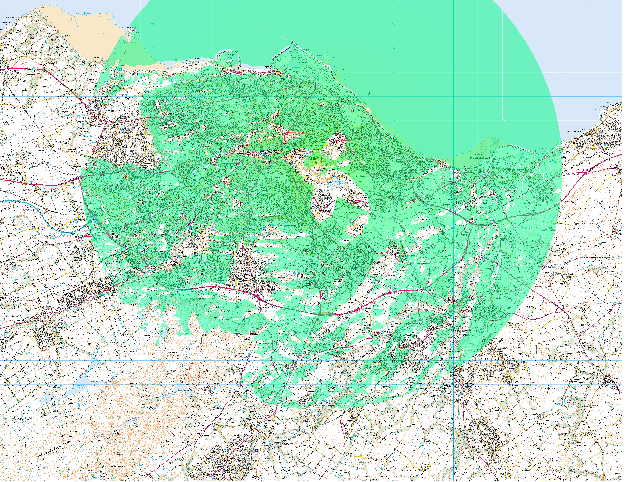
Now, let’s compute a viewshed from the top of Arthur’s seat which, in British National Grid coordinates, is at (327529.027, 672952.178). We do this with the r.los command.

r.los input=profile-dtm output=arthur_seat \
    coordinate=327529.027,672952.178 obs_elev=2 max_dist=1000

This computes the viewshed from 2m above the surface out to a maximum of 1km.

This may or may not work and may or may not have errors. It is also slow. The r.viewshed Add-on does better. It means you need to have GRASS compiled with C++ (–enable-cxx) and probably largefile (–enable-largefile) support.

There also seems to be a minor installation bug that stops extensions from being properly installed. It can be fixed by doing,

mv /usr/local/grass-6.4.3RC2/tools/g.html2man tmp.$$
mv tmp.$$/g.html2man /usr/local/grass-6.4.3RC2/tools/g.html2man
rmdir tmp.$$

So then you can install the extension from within GRASS by doing

g.extension extension=r.viewshed

and it will download and install it. The r.viewshed command takes almost exactly the same arguments as r.los, plus a few more because it’s can do more sophisticated analysis. To start, having perhaps run r.los already to see how slow it is,

r.viewshed input=profile-dtm output=arthur_seat \
    coordinate=327529.027,672952.178 obs_elev=2 max_dist=10000 \
    --overwrite 

the last argument causing the result layer to be overwritten if it already exists.

The result is something that can be displayed like this: